Rémi Flamary
Professional website
 English
 Français
 Zorglangue
Discrete optimal transport
$$ \newcommand{\argmin}{\mathop{\mathrm{arg\,min}}} \def\X{ {\bf X} } \newcommand{\G}{ {\boldsymbol{\gamma}} } \newcommand{\Gzero}{ {\boldsymbol{\gamma} }_{0}} \def\C{ {\bf C} } \newcommand{\x}{ {\bf x} } \newcommand{\w}{ {\bf w} } \newcommand{\y}{ {\bf y} } \newcommand{\xsi}{ {\bf x}^s_i} \renewcommand{\xi}{ {\bf x}_i} \newcommand{\xti}{ {\bf x}^t_i} \newcommand{\xtj}{ {\bf x}^t_j} \def\R{\mathbb{R} } \def\Pp{\bf \mathcal{P} } \newcommand{\T}{ {\bf T} } \newcommand{\diag}{\text{diag}} $$
Short introduction to optimal transport (OT)
Data and definitions
OT aims at computing a minimal cost transportation between a source probability distribution $\mu_s$, and a target distribution $\mu_t$. Here we consider the case when those distributions are only available through a finite number of samples, and can be written as
where $\delta_{\xi}$ is the Dirac at location $\xi \in \mathbb{R}^d$. $p^s_{i}$ and $p^t_{i}$ are probability masses associated to the $i$-th sample, belonging to the probability simplex, i.e. $\sum_{i=1}^{n_s} p^s_{i} = \sum_{i=1}^{n_t} p^t_{i} = 1$. The source and target samples are in matrices $\X_s=[\x_1^s,\dots,\x_{ns}^s]^\top\in\R^{n_s\times d}$ and $\X_t=[\x_1^t,\dots,\x_{ns}^t]^\top\in\R^{n_s\times d}$, respectively. The set of probabilistic couplings between these two distributions is then the set of doubly stochastic matrices $\Pp$ defined as
where $ \mathbf{1}_{d}$ is a d-dimensional vector of ones.
Optimisation problem
The Kantorovitch formulation of the optimal transport is:
where $\left< .,. \right>_F$ is the Frobenius dot product and $\C \geq 0$ is the cost function matrix of term $C(i,j)$ related to the energy needed to move a probability mass from $\xsi$ to $\xtj$. In our setting, this cost is chosen as the Euclidian distance between the two locations, i.e. $C(i,j) = ||\xsi - \xtj||^2$, but other types of metric could be considered, such as Riemannian distances over a manifold.
One can also add a regularization term to the optimal transport. In this case the problem becomes
where $\Omega(\G)$ is a regularization term that can be for instance an entropy-based regularization such as
This term has been recently proposed by Cuturi [2] as a way to regularize the transport and the optimization problem is much more easy to solve thanks to an efficient algorithm called Sinkhorn-Knopp.
Interpolation
When the optimal transportation plan $\G$ has been estimated,one can interpolate the distributions from the source to the target. The natural interpolation corresponds to a displacement of the diracs from the source to target distribution
where $t\in[0,1]$ is the parametrizes the transport from the source distribution $\mu_s$ (when $t=0$)to the target distribution $\mu_t$ (when $t=1$ ).
One can also transport the source distribution by expressing the new transported distribution $\hat{\bf X}_s$ as linear combination of elements from $\X_t$. The transportation of the source samples $\X_s$ onto that target samples $\X_t$ is computed with:
The interpolation is then expressed as
Those two interpolations have been used in numerous publisations and are illustrated in the following.
Demo
We illustrate the OT problem solution and resulting interpolation for a simples 2D dataset in the following. In this particular case the number of source and target samples are equal and the probability masses are all equal to .
Data set
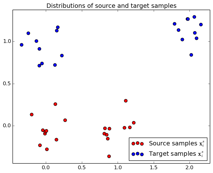
On the left, we plot the 2D position of the toy example, when the mouse pointer is on the image, you can see the index of each point. On the right, the corresponding cost matrix $\mathbf{C}$, the xias correspond to the index of the samples on the right.
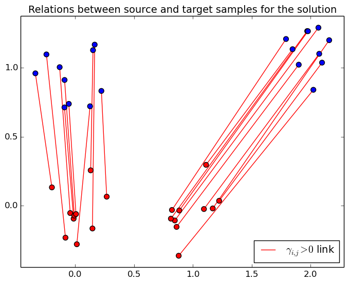
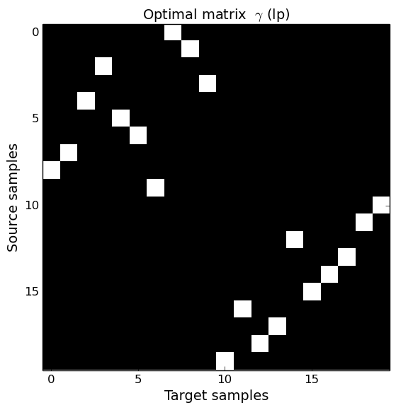
Problem solution
Interpolation
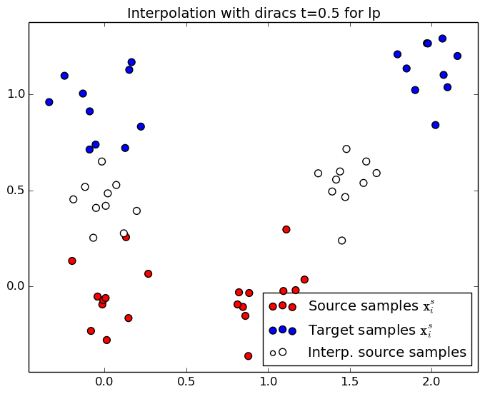
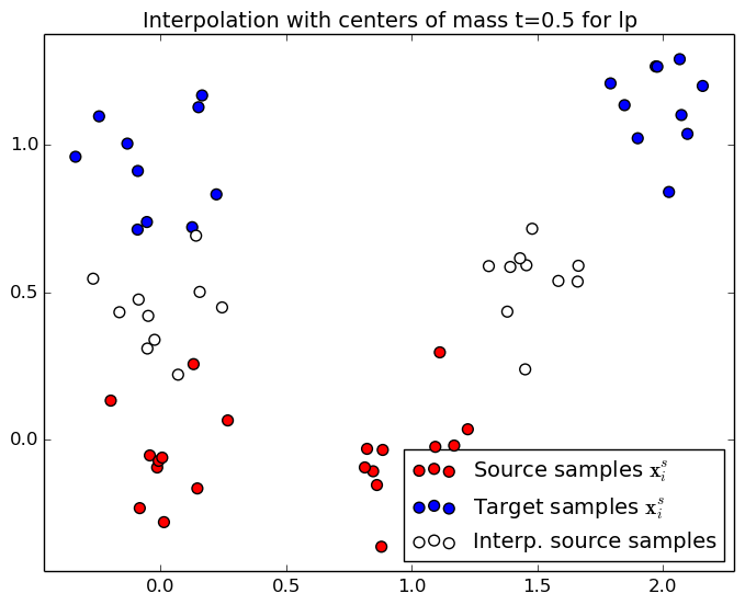
This section illusttrate the two interpolation procedures (diracs and cernter of mass) for two different regularization scheme. When no regularization is used, the solution is a permutation matrix and the mass is tranfered from a unique source sample to a unique target sample. When an entropic regularization is used, the transportation matrix is not sparse anymore and the mass is spread onto several target samples. Use the controls at the end of the page to change the optimal transport regularization and interpolation time $t\in[0,1]$.
References
A complete reference to Optimal Transport has been writtten by C. Villani [1] and is available on the web. The entropic regularization has been proposed in the machine learning community by M. Cuturi [2]. Other regularization such as Laplacian regularization have been proposed in [3].
[1] C. Villani. Optimal transport: old and new. Grundlehren der mathematischen Wissenschaften. Springer, 2009.
[2] M. Cuturi. Sinkhorn distances: Lightspeed computation of optimal transportation. In NIPS, pages 2292–2300. 2013.
[3] S. Ferradans, N. Papadakis, J. Rabin, G. Peyré, and J.-F. Aujol. Regularized discrete optimal transport. In Scale Space and Variational Methods in Computer Vision, SSVM, pages 428–439, 2013.